Structured Spreadsheet Modelling and Implementation with Multiple Dimensions

Proceedings of the EuSpRIG 2017 Conference “Spreadsheet Risk Management” ISBN : 978-1-905404-54-4

Structured Spreadsheet Modelling and Implementation

with Multiple Dimensions - Part 1: Modelling

Paul Mireault

Founder, SSMI International

Honorary Professor, HEC Montréal



Paul.Mireault@SSMI.International

ABSTRACT

Dimensions are an integral part of many models we use every day. Without thinking about it, we frequently use

the time dimension: many financial and accounting spreadsheets have columns representing months or years.

Representing a second dimension is often done by repeating blocs of formulas in a worksheet of creating

multiple worksheets with the same structure.

1 Introduction

Most organizations deal with dimensions, without calling them as such. For example:

• Products, product categories, product types.

• Clients, client types, client status.

• Markets or sectors, like education or health.

• Locations. They may be geographical (such as countries, continents, regions) or specific

(such as manufacturing plants, warehouses) or arbitrary (such as sales regions).

In this paper, we will first present some examples of multidimensional spreadsheets. Then, we will do

a brief summary of the conceptual modelling methodology we use to represent the problem we wish

to solve with a spreadsheet. We will then present basic concepts of dimensions, variables and

multidimensional expressions. We conclude with a case study and describe its complete

multidimensional model.

2 Examples of multidimensional spreadsheets

Microsoft Excel has a tool called Pivot Table that can help the spreadsheet developer present a

multidimensional dataset in a two-dimensional table, using rows and columns to represent more than

one dimension. While Pivot Tables are good for presenting data, they are less suited for presenting

business spreadsheets. The principal reason is that Pivot Tables require that their source is organized

vertically as tables: each column represents a variable, and the rows represent the repeated values.

The spreadsheets we are interested in are organized horizontally: the rows represent variables and the

columns are the repeated values. We could transpose an horizontal structure into a vertical one, but

this extra step does not alleviate Pivot Table’s other shortcoming. The major reason we feel that Pivot

Tables are not suitable for spreadsheet that represent a model used to analyse scenarios, as opposed to

a spreadsheet containing data, is that they do not update their results when their base data changes.

For that reason, the results produced by Pivot Tables cannot be used in the calculations of other

variables.

Even though a spreadsheet has two dimensions, rows and columns, it usually represents only one

dimension. Most business spreadsheet use rows for variables, leaving the columns for one dimension,

like the Time dimension.

One approach is to create one worksheet for each instance of a dimension and implementing the other

dimensions inside those worksheets. For example, if the dimension is Region, there could be four

worksheets for North, East, West and South. One could then build a fifth worksheet with

consolidating formulas.

Proceedings of the EuSpRIG 2017 Conference “Spreadsheet Risk Management” ISBN : 978-1-905404-54-4

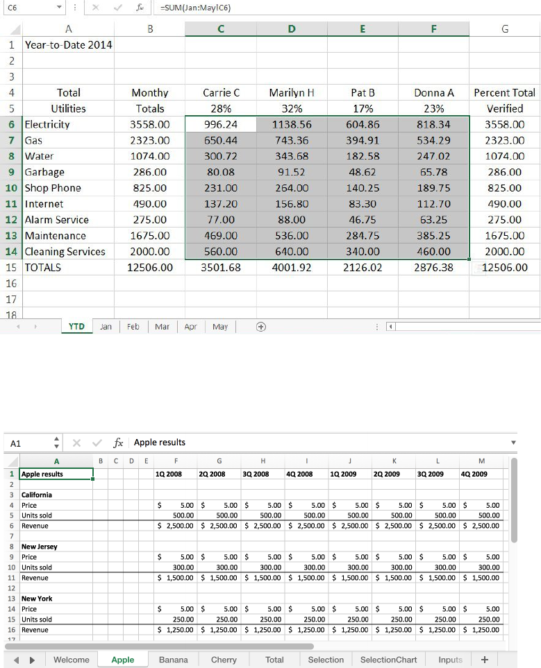
This method is proposed by (Sartain, 2014) where the author describes using 13 worksheets, one for

each month and one for consolidation, and each worksheet assigns expense variables, in rows, to

different persons, in columns (see Figure 1). The author also describes the maintenance task of adding

or removing an account, which involves performing the same operation 13 times, once for each

worksheet. She also strongly suggests, when adding an account, to add the row somewhere in the

middle of the other accounts to make sure that the subtotal row includes it in its calculation.

Figure 1 Multidimensional spreadsheet example from (Sartain, 2014)

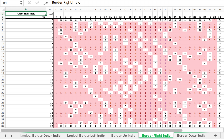
(Brandewinder, 2008) has a spreadsheet with three dimensions: Quarter, Product and Region (see

Figure 2). The Product dimension is presented as different worksheets, the Quarter dimension as

columns and the Region dimension as blocs of repeated formulas.

Figure 2 Multidimensional spreadsheet example from (Brandewinder, 2008)

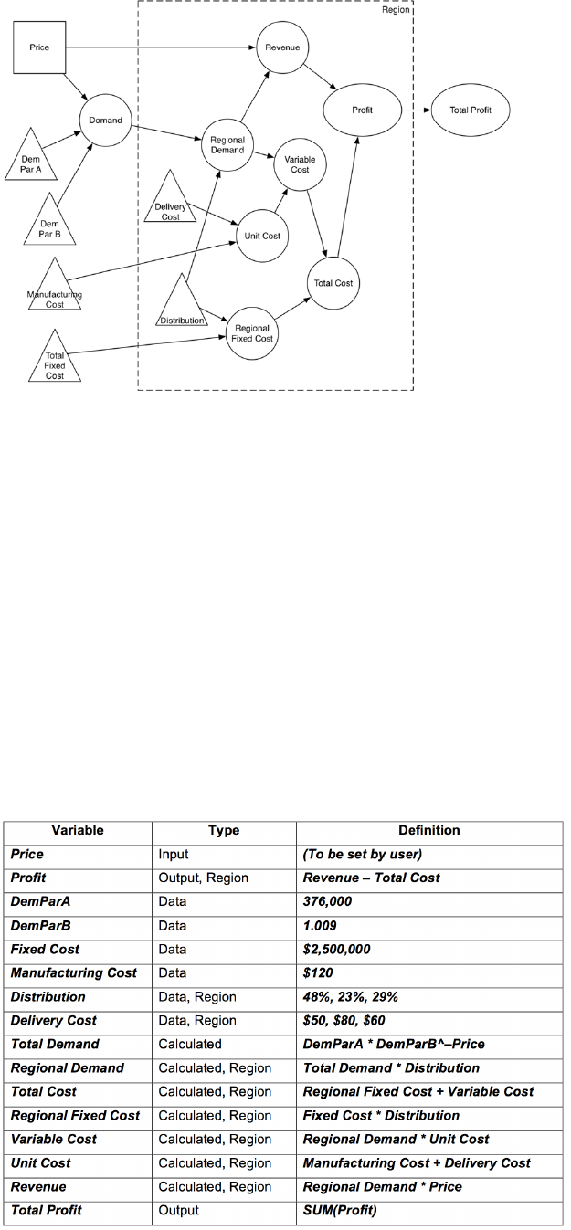
One can use an entire worksheet to represent one two-dimensional variable. Figure 3 shows an

unpublished example where the two-dimensional variable Border Right Indic is implemented in its

own worksheet.

Proceedings of the EuSpRIG 2017 Conference “Spreadsheet Risk Management” ISBN : 978-1-905404-54-4

Figure 3 Example of a worksheet used for one two-dimensional variable

(Savage, 1997) describes two important problems with using dimensions in spreadsheets. First is

scalability, which involves changing the cardinality of a dimension. He concludes that spreadsheets

rarely scale well. Second is hyper-scalability, which involves changing the dimensions themselves,

such as adding more dimensions. His conclusion is, succinctly, “Forget it”.

Multi-dimensional spreadsheets have also been used in specific optimization problems. (Kumar,

2014) describes a course scheduling problem with three dimensions: faculty, course and timeslot. A

textbook by (Powell & Baker, 2013) presents many classic Management Science problems such as the

Network Flow, the Assignment and the Traveling Salesman. While they present some multi-

dimensional problems, their spreadsheets are specific to each problem.

3 The Conceptual Model

In Information Systems development, the stage were the requirements are specified produces the

conceptual model. The conceptual model describes what the system must do, with little reference to

the technology that will be used for the implementation.

(Grossman & Özlük, 2010) in their study of three spreadsheet engineering methodologies found that

two of them do not discuss modeling and the other requires a detailed output specification.

Other researchers described building a conceptual model before implementing the spreadsheet, even

though they did not call it conceptual modelling. The Jackson Structured Diagram, a diagraming

technique based on programming concepts, has been proposed by (Knight, Chadwick, &

Rajalingham, 2000). Their diagram has some similarities with the simple Formula Diagram of

(Mireault, 2017), but they do not show how to extend it to a one dimension model. (Powell & Baker,

2013) use Influence Charts to model a problem and give general advice on how to implement it in a

spreadsheet. While their examples show a one-dimension spreadsheet, with Quarters, their Influence

Chart does not show which variables belong to the Quarter dimension.

3.1 The Formula Diagram of the SSMI Methodology

(Mireault, 2017) presents a methodology for developing spreadsheets based, primarily, on following

the process used in information systems development, where the requirement specifications is

separate from the implementation. The Structured Spreadsheet Modelling and Implementation (SSMI)

methodology consist of building a conceptual model of the spreadsheet’s variables and their formulas

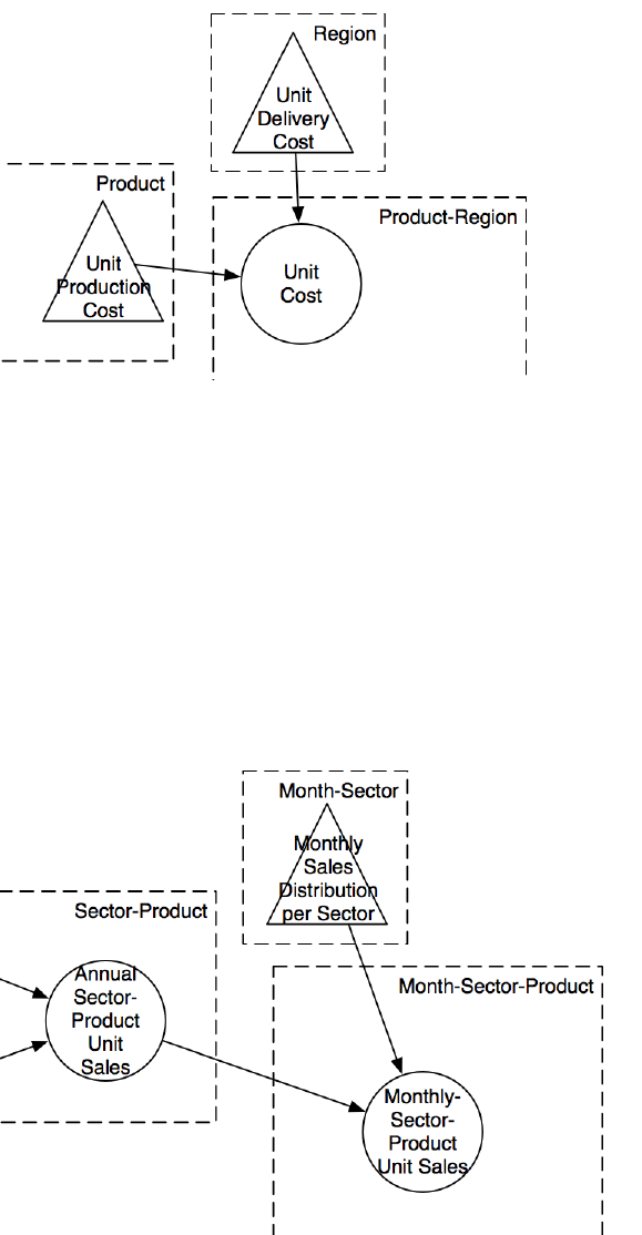
before doing the implementation. The conceptual model is composed of a Formula Diagram (Figure

4) and a Formula List (Figure 5), and they are used later to do the implementation of the spreadsheet.

Proceedings of the EuSpRIG 2017 Conference “Spreadsheet Risk Management” ISBN : 978-1-905404-54-4

Figure 4 Example of a Formula Diagram, taken from (Mireault, 2017)

The Formula Diagram uses the following symbols:

• Triangles and squares represent data values. The squares are used for input values, data that

the developer wants to implement in an Interface worksheet to allow the user to easily modify

its value. The other data, the triangles, represent data that don’t change often and will be

implemented in their own specific data worksheets.

• Circles and ovals represent calculated variables. The ovals are used for results that the

developer wants to display in the Interface worksheet, close to the input data so the user can

quickly see the impact of changing an input value. The circles are variables of less interest to

the user and are implemented in their own specific model worksheets.

• Arrows indicate which variables are involved in the calculation of the variable receiving

them.

• The dash-bordered box represents a dimension, also called entity. All the variables appearing

within the box have multiple values, one value for each instance of the repeated entity. For

example, if we have three regions, then the variable Regional Demand has three values. All

the variables appearing outside the dashed box have a single value.

Figure 5 Example of a Formula List

Proceedings of the EuSpRIG 2017 Conference “Spreadsheet Risk Management” ISBN : 978-1-905404-54-4

While the Formula Diagram gives a global view of the model, the corresponding Formula List gives a

detailed view, with all the formulas written in an Excel-like form, using variable names.

The Formula Diagram is inspired from the Influence Diagram, as presented in (Bodily, 1985). The

Influence Diagram has a richer set of modeling concepts, such as uncertainty in the values of data

variables and uncertainty in the formulas of calculated variables. But the Influence Diagram has no

representation of groups of repeating variables, which the Formula Diagram represents with a dash-

bordered box.

4 Multidimensional modelling concepts

At this point, we invite the reader to read the case study presented in the appendix so that they can get

a better appreciation of the concepts we present in this section.

4.1 Dimensions

A dimension is a set of values that serve to characterize a specific value. The set of values form a

partition. A partition, in set theory, represent subsets whose intersections, taken two by two, are null,

and whose union is the universal set, that is the set of all values. In plain language, it means that there

is no overlap and all possibilities are covered.

For example, if we use the dimension Region to characterize clients and we have the set of values

{Mountain, Valley, Lake}, a client must belong to one of the regions (all possibilities are covered)

and cannot belong to two regions (no overlap).

4.2 Dimension sets

A dimension set is a set comprised of 0 or more dimension, and a variable belongs to a specific

dimension set. Often, the variable name we use gives a clue to the dimension set it belongs to: the

variable named Monthly Production belongs to the dimension set (Month) and the variable Monthly

Regional Sales belongs to the dimension set (Month, Region).

We will say that a variable belonging to the empty, (), dimension set is dimensionless. We will also

say that dimension sets composed of only one dimension are basic. Finally, the dimension set

composed of all the dimensions is called the full dimension set.

If we have ! dimensions, then we have "

possible dimension sets, ranging from the empty set to the

set of all dimensions. Thus, when we have only one dimension, like Time, a variable either belongs to

the (Time) dimension set or is dimensionless. If we have two dimensions, like Month and Region, a

variable either belongs to the (Month, Region) dimension set, the (Month) dimension set, the (Region)

dimension set or the () dimension set.

4.3 Defining variables

In usual mathematical notation, a variable’s dimension set is indicated by subscripts. Thus, the two

variables described above would be written like this:

$%&'()*+,-%./0'1%&

$%&'(

and

$%&'()*+2341%&5)+65)37

89:;<=>?@A9:

. It is redundant to specify the dimension set in the variable’s

name and in the subscripts: we will only do so in this section because we want to make sure that the

dimensions are clear.

There are mathematical rules to remember when dealing with expressions involving variables of

different dimension sets. We usually apply them without thinking about it because they are common

sense. We will describe the rules and show how they are represented in a Formula Diagram and a

Formula List.

Rule 1: The dimension set of a formula is the union of the dimension sets of all the variables that are

part of its definition.

Example 1:

• Unit Production Cost is of dimension set (Product).

• Unit Delivery Cost is of dimension set (Region).

Proceedings of the EuSpRIG 2017 Conference “Spreadsheet Risk Management” ISBN : 978-1-905404-54-4

• Unit Cost = Unit Production Cost + Unit Delivery Cost is thus of dimension set (Product,

Region).

• The mathematical representation of the formula is:

B&1'+C%7'+

,-%./0'=+2341%&

D B&1'+,-%./0'1%&+C%7'+

,-%./0'

E B&1'+F3)1G3-*+C%7'+

2341%&

• Figure 6 illustrates how this variable definition is shown in a Formula Diagram.

Figure 6 Defining a two-dimensional variable from two one-dimensional variables

Example 2:

• Annual Sector-Product Unit Sales is of dimension set (Sector, Product).

• Monthly Sales Distribution per Sector is of dimension set (Month, Sector).

• Monthly-Sector-Product Unit Sales = Annual Sector-Product Unit Sales * Monthly Sales

Distribution per Sector is thus of dimension set (Month, Sector, Product).

• The mathematical representation of the formula is:

$%&'()*H630'%-H,-%./0'+B&1'+65)37+

$%&'(=+630'%-=+,-%./0'

D I&&/5)+630'%-H,-%./0'+B&1'+65)37+

630'%-=+,-%./0'

E $%&'()*+65)37+F17'-1J/'1%&+K3-+630'%-+

$%&'(=+630'%-

• This is shown in Figure 7.

Figure 7 Defining a three-dimensional variable from two two-dimensional variables

Rule 2: Besides aggregation, a variable can only be defined with variables having a dimension set that

is a subset of its own.

Proceedings of the EuSpRIG 2017 Conference “Spreadsheet Risk Management” ISBN : 978-1-905404-54-4

Example:

• Monthly-Sector-Product Unit Sales is of dimension set (Month, Sector, Product)

• It can be defined with variables of dimension sets (Month, Sector, Product), (Month, Sector),

(Month, Product), (Sector, Product), (Month), (Sector), (Product) and ().

• It cannot be defined with variables of dimension sets (Month, Region) or (Product, Region)

• Figure 6 and Figure 7 are also illustrations of this rule.

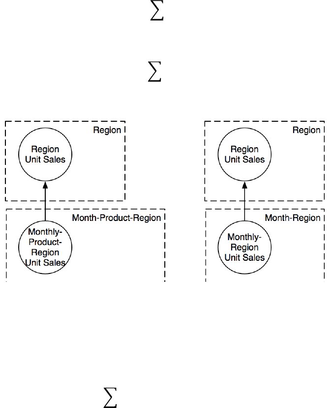
Rule 3: In the case of an aggregation, a variable can only be defined with a variable having a

dimension set that is a superset of its own.

Example 1:

• Regional Unit Sales is of dimension (Region).

• It can be aggregated from a variable of dimension sets (Month, Product, Region), (Sector,

Region) or (Month, Region).

• It cannot be aggregated from a variable of dimension sets (Month, Sector) or (Product).

• In the Formula List, we would write it as =SUM(Monthly-Product-Region Unit Sales) or

=SUM(Monthly-Region Unit Sales). Mathematically, both formulas are equivalent.

• The mathematical representations of the two formulas are:

2341%&5)+B&1'+65)37

2341%&

D $%&'()*H,-%./0'H2341%&+B&1'+65)37+

$%&'(=+,-%./0'=+2341%&

$%&'(+

,-%./0'

2341%&5)+B&1'+65)37

2341%&

D $%&'()*H2341%&+B&1'+65)37+

$%&'(=+2341%&

$%&'(

• Figure 8 shows how we would present the two formulas in the Formula Diagram.

Figure 8 Two ways to define the same aggregate variable

Example 2:

• Regional-Product Unit Sales is of dimension set (Product, Region).

• It can be aggregated from a variable of dimension sets (Month, Product, Region), (Sector,

Product, Region) or (Month, Sector, Product, Region).

• The mathematical representation of the formula is:

2341%&5)H,-%./0'+B&1'+65)37

,-%./0'=+2341%&

D $%&'()*H,-%./0'H2341%&+B&1'+65)37+

$%&'(=+,-%./0'=+2341%&

$%&'(

• It cannot be aggregated from a variable of dimension sets (Month, Region) or (Product).

Proceedings of the EuSpRIG 2017 Conference “Spreadsheet Risk Management” ISBN : 978-1-905404-54-4

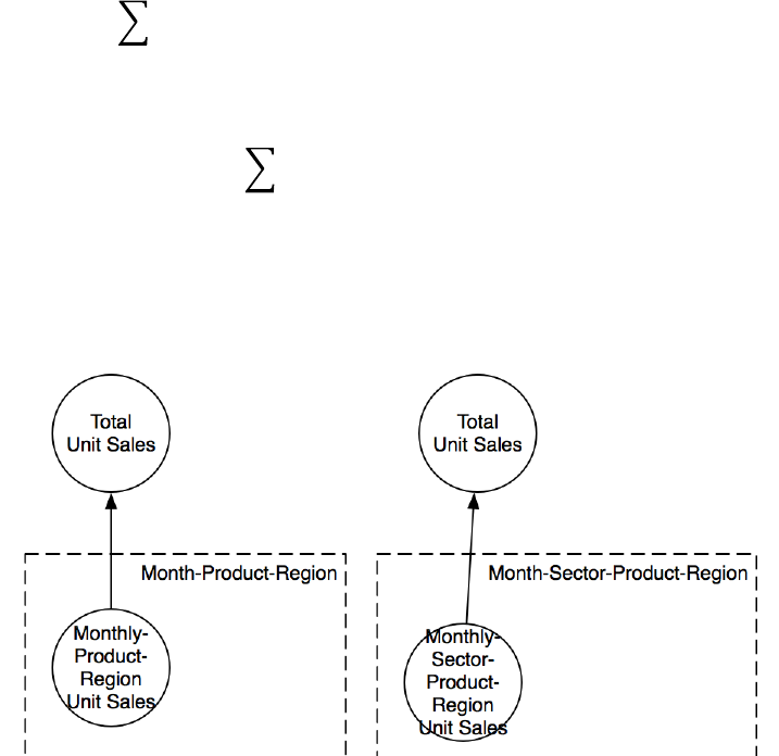
Example 3:

• Total Unit Sales is of dimension set ().

• It can be aggregated from a variable of any dimension set.

• In the Formula List, we would write it as =SUM(Monthly-Sector-Product-Region Unit

Sales) or =SUM(Monthly-Product-Region Unit Sales). Mathematically, both formulas are

equivalent.

• The mathematical representations of the two formulas are:

L%'5)+B&1'+65)37

D $%&'()*H630'%-H,-%./0'H2341%&+B&1'+65)37+

$%&'(=+630'%-=+,-%./0'=+2341%&

$%&'(

+630'%-+

,-%./0'+

2341%&

L%'5)+B&1'+65)37 D $%&'()*H,-%./0'H2341%&+B&1'+65)37+

$%&'(=+,-%./0'=+2341%&

$%&'(

,-%./0'+

2341%&

In the Formula Diagram, the dimensionless variable is shown outside of any box, as illustrated in

Figure 9.

Figure 9 Defining a dimensionless variable as an aggregate of a multidimensional variable

5 Conclusion

In this paper, we extended the one-dimension conceptual model of (Mireault, 2017) to model a

multidimensional problem. By building the conceptual model before doing the implementation, the

spreadsheet developer is not trying to solve two different problems at the same time: How do I

calculate this variable? and How do I implement this in my spreadsheet?

An experiment by (O'Donnel, 2001) showed that using a diagramming technique, an Influence

Diagram in this case, did not take significantly more time to produce the final spreadsheet and those

spreadsheets had significantly less errors of the type “omitted factors” than those of the control group.

The problem submitted to the test subjects was a relatively simple one, with one time dimension of

two periods. It would be interesting to reproduce the experiment with a more complex multi-

dimensional problem such as the one presented in the Appendix.

Part 2 of this paper will present a structured methodology to implement the multidimensional model.

Proceedings of the EuSpRIG 2017 Conference “Spreadsheet Risk Management” ISBN : 978-1-905404-54-4

Appendix – Case Study

In this section, we present a pedagogical case study to illustrate the concepts presented in this paper.

The solution is not unique: there are many ways of calculating some variables, as illustrated above.

The Acme TechnoWidget Company

The Acme TechnoWidget Company produces and sells widgets. It produces two products (a Standard

widget and a Deluxe widget) and its salesforce is assigned to four major sectors: Government,

military, education and private.

Market research has established that the annual demand for widgets depends on each sector’s

Standard widget price. The Pricing Director explains:

We start by setting a global base price. Then, for each sector, we tell our salesforce that they can

offer a rebate. For instance, we offer a 70% rebate to the education sector and it’s 10% for the

private sector because purchases are usually made by researchers with limited funds. The military

sector gets a 20% rebate and the government 40%. This is not made public: all our price lists show

the base price, but our clients in each sector are aware of the rebate they can get.

Each sector reacts differently to a change of price. We consulted with a market research expert and

she came up with multiple demand functions, one for each sector. The demand function estimates a

sector’s annual demand for a given base price. The demand function has the form M ,-103

. The

parameters O and M are different for each sector, and ,-103 is the sector’s price, after the rebate.

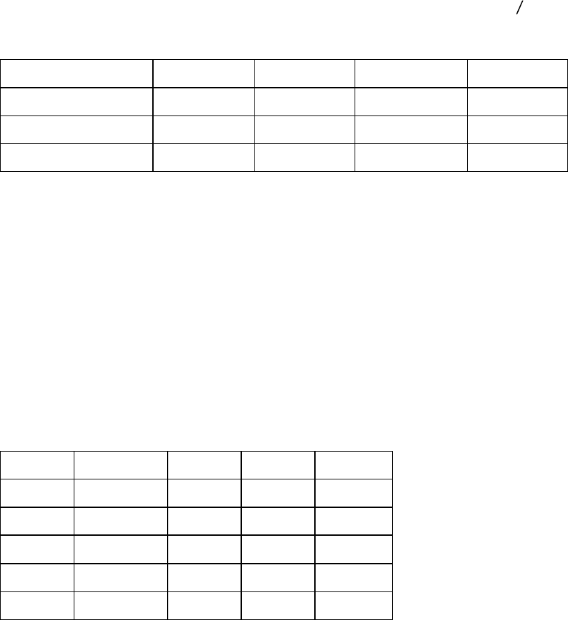
This table shows the values the expert gave us:

Sector'

Government'

Military'

Private'

Education'

Rebate&Percentage&

40%&

20%&

10%&

70%&

DemParA&

3.593437587&

3.46315031&

3.187228762&

4.114496316&

DemParB&

22858963442&

The price of the Deluxe widget is 45% higher than the Standard widget.

The Sales Manager explains the sales pattern:

The annual demand of each Sector is split between the Standard and Deluxe product types, but the

distribution is very different in each sector. For instance, in the education sector, with its limited

funds, the split is 80%-20% and it is 25%-75% in the military sector. I guess these guys always go for

the best, and they have higher budgets. The distribution is 65%-35% for the government sector and

40%-60% for the private sector. The ratios are then applied to the sector’s annual demand to get the

annual demand by product.

Another interesting pattern is the distribution of sales during the year. We noticed that our clients buy

more just before the end of their fiscal year, when some want to spend their budget surpluses, and the

beginning, when others have new funds allotted. Each sector has a different pattern, and we noticed

that it is pretty stable year after year.

Government'

Military'

Private'

Education'

Jan'

9%'

8%'

12%'

6%'

Feb'

10%'

9%'

11%'

8%'

Mar'

12%'

10%'

9%'

Apr'

12%'

7%'

10%'

May'

11%'

13%'

6%'

12%'

Proceedings of the EuSpRIG 2017 Conference “Spreadsheet Risk Management” ISBN : 978-1-905404-54-4

Jun'

9%'

11%'

4%'

12%'

Jul'

7%'

9%'

5%'

11%'

Aug'

6%'

7%'

6%'

9%'

Sep'

5%'

6%'

8%'

7%'

Oct'

5%'

4%'

9%'

6%'

Nov'

6%'

5%'

11%'

5%'

Dec'

8%'

6%'

12%'

5%'

Total'

100%'

Sales to a sector are not uniformly distributed by region. For example, there are more universities in

the South-West than in the West. The following table shows the distribution of a sector’s sales by

region. With it, we can calculate the expected monthly sales per product per region, which helps our

Logistics Department do its planning.

Government'

Military'

Private'

Education'

25%'

52%'

22%'

24%'

SE'

18%'

13%'

21%'

15%'

SW'

18%'

17%'

32%'

22%'

0%'

25%'

17%'

15%'

12%'

Total'

100%'

The costs of producing a widget are $48 and $72 for the Standard and the Deluxe widget respectively.

The monthly fixed costs for this year are $20000. Delivery costs depend solely on the region and are

shown in this table:

Region'

North'

South-East'

South-West'

East'

West'

Unit&Delivery&Cost&

$10.25&

$9.73&

$9.58&

$8.26&

$11.02&

The company CEO wants to see the following results:

• The monthly sales amount and units per product.

• The monthly units, sales amount, costs and profit.

• The total profit.

Proceedings of the EuSpRIG 2017 Conference “Spreadsheet Risk Management” ISBN : 978-1-905404-54-4

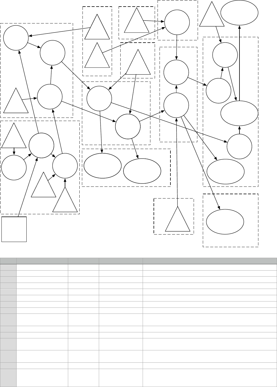
Acme TechnoWidget Company Formula Diagram

Acme TechnoWidget Company Formula List

Variable

Type

Dimension Set

Value / Formula

Base Price

Input

100

Base Price Multiplier

Data

Product

(1, 1.45)

Unit Production Cost

Data

Product

list of values

Rebate Percentage

Data

Sector

list of values

Sector Price Factor

Calculated

Sector

1-Rebate Percentage

Sector Base Price

Calculated

Sector

Base Price * Sector Price Factor

DemParA

Data

Sector

list of values

DemParB

Data

Sector

list of values

Sector Annual

Demand Units

Calculated

Sector

DemParA*DemParB^-Sector Base Price

Unit Delivery Cost

Data

Region

list of values

PR Unit Cost

Calculated

Product-Region

Unit Production Cost + Unit Delivery Cost

Product Distribution

per Sector

Data

Sector-Product

list of values

Annual Sector-

Product Unit Sales

Calculated

Sector-Product

Sector Annual Demand Units * Product Distribution per

Sector

Price

Calculated

Sector-Product

Sector Base Price * Base Price Multiplier

Annual Sector-

Product Sales

Amount

Calculated

Sector-Product

Annual Sector-Product Unit Sales * Price

Month

Month-Sector-

Product-Region

Region

Product

Sector

Sector-Product

Product-Region

Month-Sector

Sector-Region

Rebate

Percentage

Unit

Production

Cost

DemParA

Unit

Delivery

Cost

Monthly

Fixed

Cost

Sector

Price

Factor

Price

Unit

Cost

MSPR

Unit

Sales

MSPR

Variable

Cost

Monthly

Variable

Cost

Monthly

Cost

Monthly

Sales

Amount

Monthly

Proﬁt

Annual

Sector-

Product

Sales

Amount

Annual

Sector-

Product

Unit

Sales

Region

Sales

Distribution

per Sector

Product

Distribution

per Sector

Monthly

Sales

Distribution

per Sector

Base

Price

Multiplier

Sector

Base

Price

MSP

Unit Sales

Sales Amount

Base

Price

Multiplier

Sector

Base

Price

DemParB

Sector

Annual

Demand

Units

Month-Sector-Product

MSP

Unit Sales

MSP

Sales

Amount

Monthly

Unit

Sales

Month-Product-Region

MPR

Unit Sales

Month-Product

Unit Sales

Sales Amount

Total

Proﬁt

Base

Price

Proceedings of the EuSpRIG 2017 Conference “Spreadsheet Risk Management” ISBN : 978-1-905404-54-4

Variable

Type

Dimension Set

Value / Formula

Region Sales

Distribution per

Sector

Data

Sector-Region

list of values

Monthly Sales

Distribution per

Sector

Data

Month-Sector

list of values

MSP Unit Sales

Calculated

Month-Sector-

Product

Annual Sector-Product Unit Sales * Monthly Sales

Distribution per Sector

MSP Sales Amount

Calculated

Month-Sector-

Product

Annual Sector-Product Sales Amount * Monthly Sales

Distribution per Sector

MSPR Unit Sales

Calculated

Month-Sector-

Product-Region

MSP Unit Sales * Region Sales Distribution per Sector

MSPR Variable Cost

Calculated

Month-Sector-

Product-Region

MSPR Unit Sales * PR Unit Cost

Monthly Variable

Cost

Calculated

Month

SUM(MSPR Variable Cost)

Monthly Unit Sales

Output

Month

SUM(MSPR Unit Sales)

Monthly Sales

Amount

Calculated

Month

SUM(MSP Sales Amount)

Monthly Fixed Cost

Data

Monthly Costs

Calculated

Month

Monthly Fixed Cost + Monthly Variable Cost

Monthly Profit

Calculated

Month

Monthly Sales Amount - Monthly Costs

MPR Unit Sales

Output

Month-Product-

Region

SUM(MSPR Unit Sales)

MP Unit Sales

Output

Month-Product

SUM(MSP Unit Sales)

MP Sales Amount

Output

Month-Product

SUM(MSP Sales Amount)

Total Profit

Output

SUM(Monthly Profit)

Proceedings of the EuSpRIG 2017 Conference “Spreadsheet Risk Management” ISBN : 978-1-905404-54-4

6 References

Bodily, S. (1985). Modern Decision Making. McGraw-Hill.

Brandewinder, M. (2008, 04 22). Excel, named ranges and INDIRECT(). Retrieved 04 27, 2017, from Clear Lines

Consulting: http://www.clear-lines.com/blog/post/Excel2c-named-ranges-and-INDIRECT().aspx

Grossman, T. A., & Özlük, O. (2010). Spreadsheets Grow Up: Three Spreadsheet Engineering Methodologies for Large

Financial Planning Models. EuSpRIG. Greenwich.

Knight, B., Chadwick, D., & Rajalingham, K. (2000). A Structured Methodology For Spreadsheet Modelling. EuSpRIG.

Kumar, R. (2014). Modeling a Department Course Scheduling Problem Using Integer Programming: A Spreadsheet-Based

Approach. Academy of Information and Management Sciences Journal, 17(2).

Mireault, P. (2017). Structured Spreadsheet Modelling and Implementation - A Methodology for Creating Effective

Spreadsheets (Second Edition ed.). Montreal: SSMI International.

O'Donnel, P. (2001). The Use of Influence Diagrams in the Design of Spreadsheet Models: an experimental study.

Australasian Journal of Information Systems, 9(1).

Sartain, J. (2014, 05 30). How to create 3D Worksheets in Excel 2013. Retrieved 04 26, 2017, from PCWorld:

http://www.pcworld.com/article/2241304/how-to-create-3d-worksheets-in-excel-2013.html

Savage, S. (1997, 02). Weighing the Pros and Cons of Decision Technology in Spreadsheets. ORMS Today, 24(1).